Pricing Method Comparison
This tutorial compares the three Fourier-based pricing methods available in OptionPricer: Carr-Madan, Lewis, and COS. All three invert the characteristic function of the log-return to price European calls, but they differ in how they handle the payoff transform, the integration contour, and the discretisation strategy. See Option Pricing for the full derivation of all three methods.
Selecting the method
Pass method when constructing the pricer:
from quantflow.options.pricer import OptionPricer, OptionPricingMethod
from quantflow.sp.heston import Heston

model = Heston.create(vol=0.2)
pricer = OptionPricer(model=model, method=OptionPricingMethod.COS)
result = pricer.maturity(1.0)
Accuracy comparison
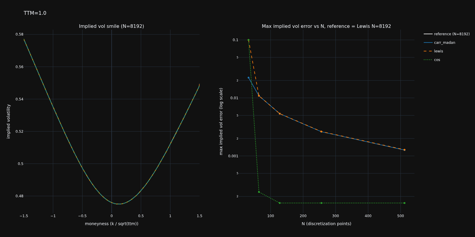
The charts below use a Heston model with \(\sigma=0.8\), \(\kappa=2\), \(\rho=-0.2\), \(\text{vol}=0.5\). The reference solution is Lewis with \(N=8192\). Implied vol errors are clipped at 10% — Lewis can produce errors well above this at low \(N\), particularly at short maturities, which would otherwise dominate the scale.
At long maturities (TTM=1.0) all three methods converge quickly:
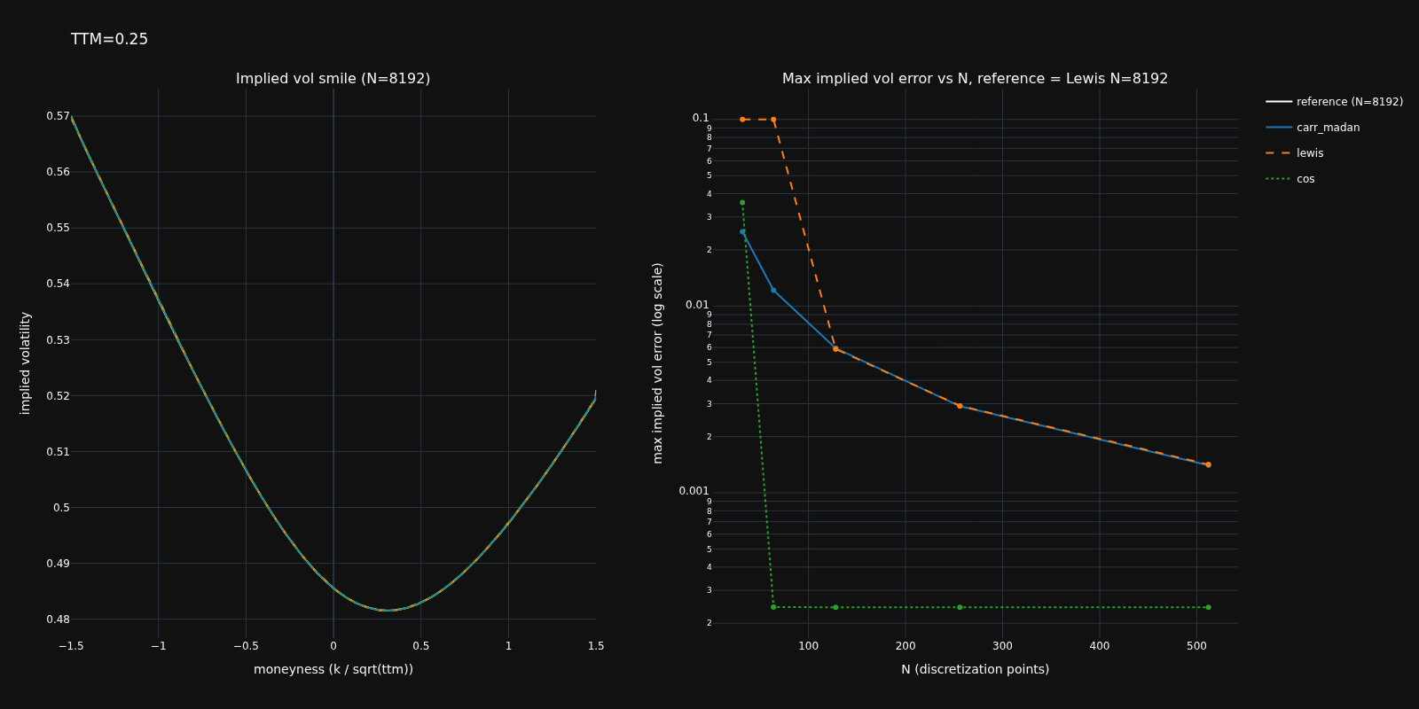
At medium maturities (TTM=0.25) COS tends to converge faster than Carr-Madan for the same \(N\):
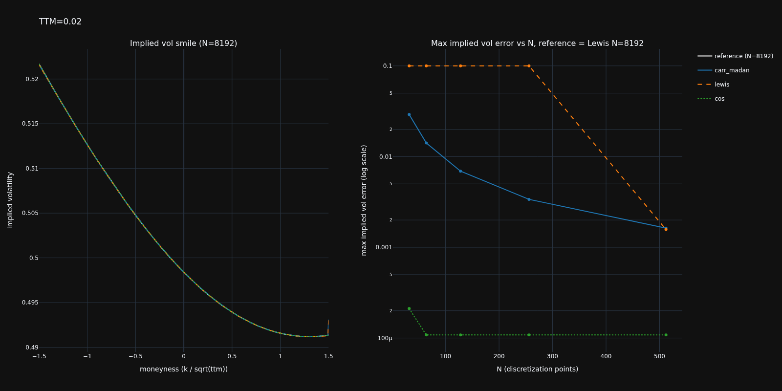
At very short maturities (TTM=0.02) the differences are most pronounced. Carr-Madan can struggle with the auto-selected \(\alpha\), while Lewis and COS remain stable:
Complexity
| Method | Complexity |
|---|---|
| Carr-Madan | \(O(N \log N)\) via Fractional Fourier Transform |
| Lewis | \(O(N \log N)\) via Fractional Fourier Transform |
| COS | \(O(N^2)\) |
Unlike the FRFT methods, COS can price a single strike at a time without computing the full grid, making it well suited for lazy or on-demand strike evaluation.
Code for the above charts
"""Compare Carr-Madan, Lewis and COS option pricing methods for accuracy."""

import numpy as np
import plotly.graph_objects as go
from plotly.subplots import make_subplots
from pydantic import BaseModel, Field

from docs.examples._utils import assets_path
from quantflow.dists.marginal1d import (
    OptionPricingCosResult,
    OptionPricingMethod,
    OptionPricingResult,
)
from quantflow.options.bs import implied_black_volatility
from quantflow.sp.base import StochasticProcess1D
from quantflow.sp.heston import Heston


class ChartProps(BaseModel):
    color: str = Field(default="#1f77b4", description="Line color for the chart")
    dash: str = Field(
        default="solid",
        description="Line dash style for the chart (e.g., 'solid', 'dash',  'dot')",
    )


class PricingMethodComparison(BaseModel):
    model: StochasticProcess1D = Field(
        description="Stochastic process model to compare"
    )
    ttms: tuple[float, ...] = Field(
        default=(1.0, 0.25, 0.02),
        description="Time to maturities to compare",
    )
    ns: tuple[int, ...] = Field(
        default=(32, 64, 128, 256, 512),
        description="Discretization points to compare",
    )
    max_moneyness: float = Field(
        default=1.5,
        description="Maximum time-adjusted moneyness for option pricing",
    )
    ref_n: int = Field(
        default=8192,
        description=(
            "Number of discretization points to use for the reference Lewis price"
        ),
    )
    max_iv_error: float = Field(
        default=0.1,
        description="Implied vol errors above this value are clipped in the error plot",
    )
    charts: dict[OptionPricingMethod, ChartProps] = Field(
        default_factory=lambda: {
            OptionPricingMethod.CARR_MADAN: ChartProps(color="#1f77b4", dash="solid"),
            OptionPricingMethod.LEWIS: ChartProps(color="#ff7f0e", dash="dash"),
            OptionPricingMethod.COS: ChartProps(color="#2ca02c", dash="dot"),
        },
        description="Chart properties for each pricing method",
    )

    def _ivs(
        self, r: OptionPricingResult, log_strikes: np.ndarray, ttm: float
    ) -> np.ndarray:
        call = np.asarray(r.call_price(log_strikes))
        intrinsic = np.maximum(0.0, 1.0 - np.exp(log_strikes))
        call = np.clip(call, intrinsic, 1.0)
        return implied_black_volatility(log_strikes, call, ttm, 0.5, 1.0).values

    def _iv_error(
        self,
        r: OptionPricingResult,
        ref: OptionPricingResult,
        log_strikes: np.ndarray,
        ttm: float,
    ) -> float:
        iv = implied_black_volatility(
            log_strikes, np.asarray(r.call_price(log_strikes)), ttm, 0.5, 1.0
        ).values
        iv_ref = implied_black_volatility(
            log_strikes, np.asarray(ref.call_price(log_strikes)), ttm, 0.5, 1.0
        ).values
        finite = np.isfinite(iv) & np.isfinite(iv_ref)
        return float(np.max(np.abs(iv[finite] - iv_ref[finite])))

    def run_ttm(self) -> None:
        for ttm in self.ttms:
            ms = self.model.marginal(ttm)
            max_log_strike = self.max_moneyness * ms.std_validated()
            log_strikes = ms.option_support(
                self.ref_n + 1, max_log_strike=max_log_strike
            )
            ref = ms.call_option(self.ref_n, max_moneyness=self.max_moneyness)
            iv_ref = self._ivs(ref, log_strikes, ttm)
            moneyness_ref = log_strikes / np.sqrt(ttm)
            ttm_label = f"TTM={ttm}"
            slug = ttm_label.lower().replace("=", "").replace(".", "_")

            fig = make_subplots(
                rows=1,
                cols=2,
                subplot_titles=(
                    f"Implied vol smile (N={self.ref_n})",
                    f"Max implied vol error vs N, reference = Lewis N={self.ref_n}",
                ),
            )
            fig.add_trace(
                go.Scatter(
                    x=moneyness_ref,
                    y=iv_ref,
                    name=f"reference (N={self.ref_n})",
                    mode="lines",
                    line=dict(color="white", width=2),
                    legendgroup="reference",
                ),
                row=1,
                col=1,
            )
            for method, props in self.charts.items():
                errors = []
                for n in self.ns:
                    r = ms.call_option(
                        n,
                        max_moneyness=self.max_moneyness,
                        pricing_method=method,
                    )
                    ks = (
                        log_strikes
                        if isinstance(r, OptionPricingCosResult)
                        else ms.option_support(n + 1, max_log_strike=max_log_strike)
                    )
                    errors.append(
                        min(self._iv_error(r, ref, ks, ttm), self.max_iv_error)
                    )
                    if n == self.ns[-1]:
                        fig.add_trace(
                            go.Scatter(
                                x=moneyness_ref,
                                y=self._ivs(r, log_strikes, ttm),
                                name=method.value,
                                mode="lines",
                                line=dict(color=props.color, dash=props.dash),
                                legendgroup=method.value,
                            ),
                            row=1,
                            col=1,
                        )
                fig.add_trace(
                    go.Scatter(
                        x=self.ns,
                        y=errors,
                        name=method.value,
                        mode="lines+markers",
                        line=dict(color=props.color, dash=props.dash),
                        legendgroup=method.value,
                        showlegend=False,
                    ),
                    row=1,
                    col=2,
                )
            fig.update_xaxes(title_text="moneyness (k / sqrt(ttm))", row=1, col=1)
            fig.update_yaxes(title_text="implied volatility", row=1, col=1)
            fig.update_xaxes(title_text="N (discretization points)", row=1, col=2)
            fig.update_yaxes(
                title_text="max implied vol error (log scale)", type="log", row=1, col=2
            )
            fig.update_layout(title=ttm_label)
            fig.write_image(
                assets_path(f"pricing_method_accuracy_{slug}.png"),
                width=1600,
                height=800,
            )


if __name__ == "__main__":
    pr = Heston.create(vol=0.5, kappa=2, sigma=0.8, rho=-0.2)
    comparison = PricingMethodComparison(model=pr)
    comparison.run_ttm()