From Characteristic Function to PDF

One uses the inverse Fourier transform formula to obtain the probability density function (PDF) from a characteristic function.

\[\begin{equation} f(x) = \frac{1}{2\pi}\int_{-\infty}^\infty e^{-iux} \Phi_x\left(u\right) du = \frac{1}{\pi} {\mathcal R} \int_0^\infty e^{-iux} \Phi_u du \end{equation}\]

The last equivalence is because the PDF is real-valued.

Discretization

The PDF integration can be approximated as:

\[\begin{align} u_m &= \delta_u m \\ f(x) &\approx \frac{1}{\pi}\sum_{m=0}^{N-1} h_m e^{-i u_m x} \Phi_x\left(u_m\right) \delta_u \end{align}\]

• \(\delta_u\) is the discretization in the frequency domain. It must be small enough to provide good accuracy of the integral.
• \(N\) is the number of discretization points and must be large enough so that the characteristic function is virtually 0 for \(u_{N-1}=\delta_u N\).
• \(h_m\) is given by the integration methodology, either trapezoidal or Simpson rule (the library supports both, with trapezoidal as default).

For full details, see Carr & Madan and Chourdakis.

One could use the inverse Fourier transform to solve the integral. However, it has \(O(N^2)\) time complexity. One alternative, implemented in the library, is using the Fast Fourier Transform (FFT), which has \(O(N \log N)\) time complexity. Another more flexible alternative is the Fractional FFT (FRFT), described in Chourdakis. This is the methodology used by default in the library.

FFT Integration

FFT is an efficient algorithm for computing discrete Fourier coefficients \(d\) from \(f\). Given an even number \(N=2^n\), these are given by

\[\begin{equation} d_j = \frac{1}{N}\sum_{m=0}^{N-1} f_m e^{-jm\frac{2\pi}{N} i}\ \ j=0, 1, \dots, N-1 \end{equation}\]

Using this formula, the discretization above can be rewritten as

\[\begin{align} x_j &= -b + \delta_x j \\ \zeta &= \delta_u \delta_x \\ f_m &= h_m \frac{N}{\pi} e^{i u_m b} \Phi_x\left(u_m\right) \delta_u\\ f(x_j) &\approx \frac{1}{N} \sum_{m=0}^{N-1} f_m e^{-j m \zeta i} \end{align}\]

The parameter \(b\) controls the range of the random variable \(x\). The FFT requires that

\[\begin{equation} \zeta = \frac{2\pi}{N} \end{equation}\]

which means \(\delta_u\) and \(\delta_x\) cannot be chosen independently — they are coupled by

\[\begin{equation} \delta_x = \frac{2\pi}{N \delta_u} \end{equation}\]

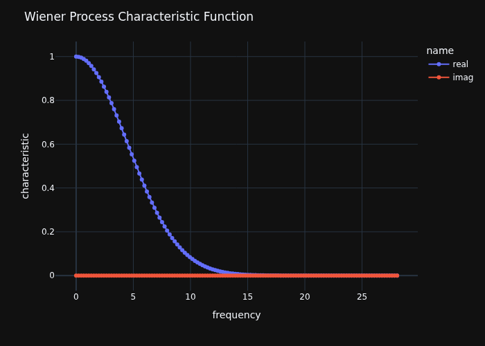
As an example, let us invert the characteristic function of the Wiener process, which yields the standard normal distribution.

from docs.examples._utils import assets_path
from quantflow.sp.wiener import WienerProcess
from quantflow.utils import plot

p = WienerProcess(sigma=0.5)
m = p.marginal(0.2)

fig = plot.plot_characteristic(m)
fig.update_layout(title="Wiener Process Characteristic Function")
fig.write_image(assets_path("wiener_characteristic.png"))

fig = plot.plot_marginal_pdf(m, n=128, use_fft=True, max_frequency=20)
fig.update_layout(title="Wiener Process PDF via FFT with n=128")
fig.write_image(assets_path("wiener_fft_128.png"))

fig = plot.plot_marginal_pdf(m, n=128 * 8, use_fft=True, max_frequency=8 * 20)
fig.update_layout(title="Wiener Process PDF via FFT with n=1024")
fig.write_image(assets_path("wiener_fft_1024.png"))

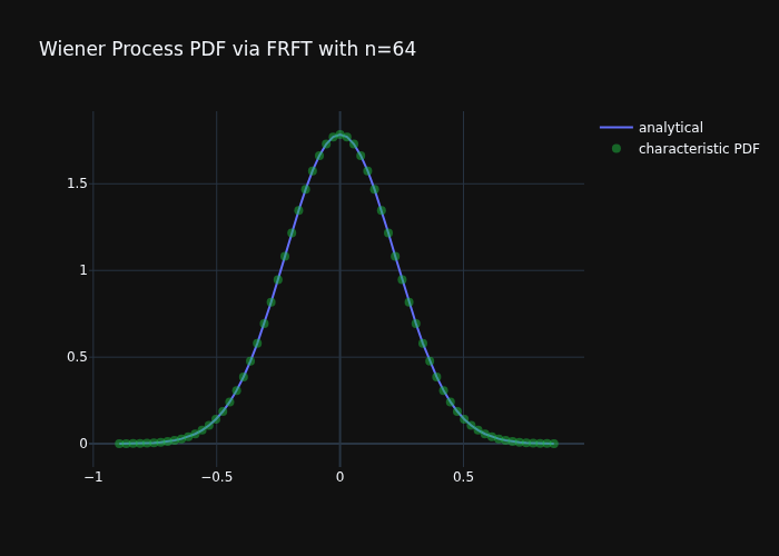
fig = plot.plot_marginal_pdf(m, 64)
fig.update_layout(title="Wiener Process PDF via FRFT with n=64")
fig.write_image(assets_path("wiener_64.png"))

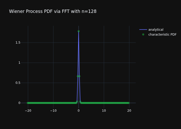
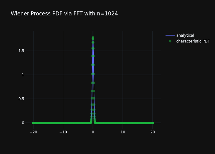
Note the amount of unnecessary discretization points in the frequency domain (the characteristic function is zero after 15 or so). However the space domain is poorly represented because of the FFT constraints (we have a relatively small number of points where it matters, around zero).

FRFT

The Fractional FFT (FRFT) is another algorithm that can be used to invert the characteristic function. Compared to the FFT, this method relaxes the constraint \(\zeta=2\pi/N\) so that the frequency domain and space domain can be discretized independently. We use the methodology from chourdakis:

\[\begin{align} y &= \left(\left[e^{-i j^2 \zeta/2}\right]_{j=0}^{N-1}, \left[0\right]_{j=0}^{N-1}\right) \\ z &= \left(\left[e^{i j^2 \zeta/2}\right]_{j=0}^{N-1}, \left[e^{i\left(N-j\right)^2 \zeta/2}\right]_{j=0}^{N-1}\right) \end{align}\]

We can now reduce the number of points needed for the discretization and achieve higher accuracy by properly selecting the domain discretization independently.

Since one N-point FRFT will invoke three 2N-point FFT procedures, the number of operations will be approximately \(6N\log{N}\) compared to \(N\log{N}\) for the FFT. However, we can use fewer points as demonstrated and be more robust in delivering results.

The FRFT is used as the default transform across the library. The FFT can be used by passing use_fft=True to the transform functions, but it is not advised.