BNS Volatility Model
This tutorial calibrates the BNS stochastic-volatility model (Barndorff-Nielsen and Shephard) and its two-factor extension BNS2 to an implied volatility surface, using the same workflow as the Heston tutorial in Volatility Surface.
BNS is structurally different from Heston. The variance process is a non-Gaussian Ornstein-Uhlenbeck process driven by a pure-jump Lévy process (Gamma-OU in this implementation), and the leverage effect is introduced by correlating the same jumps into the log-price.
Single-factor BNS
BNSCalibration fits five parameters to the surface:
| Parameter | Description |
|---|---|
v0 |
Initial variance (\(v_0\)) |
theta |
Long-run variance (\(\theta = \lambda / \beta\)) |
kappa |
Mean reversion speed of the variance process |
beta |
Exponential decay rate of the BDLP jump-size distribution |
rho |
Leverage parameter (correlation between jumps in variance and log-price) |
The BDLP intensity is set as \(\lambda = \theta \beta\) so that the stationary mean of the Gamma-OU variance process equals \(\theta\). This gives the same \((v_0, \theta)\) parameterisation as Heston.
Because the variance is built from positive jumps and exponential mean reversion, it stays positive by construction. No Feller-style penalty is needed.
How BNS fits the surface
The mechanism that produces a smile in BNS is structurally different from Heston. Heston relies on a diffusive volatility-of-variance \(\sigma\) for the wings and a spot-variance correlation \(\rho\) for the skew, both accumulating as \(\sqrt{T}\). BNS instead injects discrete jumps directly into the variance process: each jump in \(v_t\) is mirrored, scaled by \(\rho\), into the log-price. The wing thickness is governed by the jump-size distribution (controlled by \(\beta\)) and the skew by \(\rho\).
A consequence of this structural difference is that the calibrator often settles at a small \(\kappa\) together with a large \(\theta\). The time scale of mean reversion is \(1/\kappa\), so when \(\kappa\) is small the variance process barely relaxes towards \(\theta\) over the calibration horizon and stays close to \(v_0\) throughout.
In that regime \(\theta\) is only weakly identified by the surface and the optimizer can move it freely as long as the jump-driven smile dynamics are preserved. The headline number to read in the output is \(v_0\), which sets the at-the-money level.
Calibrated parameters
The fit uses the VolModelCalibration two-stage optimiser: L-BFGS-B for basin search, followed by trust-region reflective on the residual vector with parameter bounds.
xtol termination condition is satisfied.
{
  "variance_process": {
    "rate": 0.09633024176782554,
    "kappa": 3.820475670414532,
    "bdlp": {
      "intensity": 1.0078786939174174,
      "jumps": {
        "decay": 3.8233988980443363
      }
    }
  },
  "rho": -0.2952186207141647
}
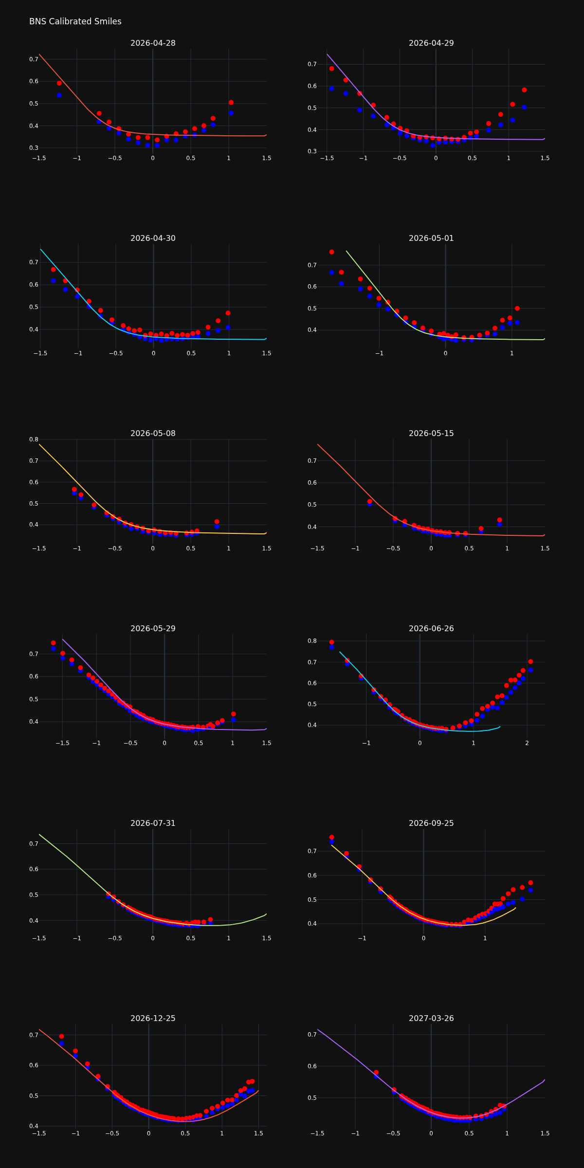
The fit is good for medium and long maturities and visibly off at the front expiries. This is the same short-maturity gap seen for Heston and Heston-jump-diffusion.
The cause here is structural: BNS adds jumps, but they live in the variance process, not directly in the log-price. The jump-driven contribution to the log-price is bounded by the size of the variance jumps multiplied by \(|\rho|\), which is small for short tenors. A model with explicit jumps in the log-price (such as HestonJ) or a rough volatility model is better suited to the steep short-term skew observed in crypto markets.
Code
import json

from docs.examples._utils import FIXTURES, assets_path, print_model
from quantflow.options.calibration import BNSCalibration
from quantflow.options.pricer import OptionPricer, OptionPricingMethod
from quantflow.options.surface import VolSurface, VolSurfaceInputs, surface_from_inputs
from quantflow.sp.bns import BNS

# Load a saved volatility surface snapshot and build the surface
with open(FIXTURES / "volsurface_btc.json") as fp:
    surface: VolSurface = surface_from_inputs(VolSurfaceInputs(**json.load(fp)))

surface.bs()
surface.disable_outliers()

# Create a BNS pricer with initial parameters
pricer = OptionPricer(
    model=BNS.create(vol=0.5, kappa=1.0, decay=10.0, rho=-0.2),
    method=OptionPricingMethod.COS,
)

calibration: BNSCalibration[BNS] = BNSCalibration(
    pricer=pricer,
    vol_surface=surface,
    moneyness_weight=0.5,
)

result = calibration.fit()
print(result.message)
print_model(calibration.model)

# Plot the calibrated smile for all maturities and save as PNG
fig = calibration.plot_maturities(max_moneyness=1.5, support=101)
fig.update_layout(title="BNS Calibrated Smiles")
fig.write_image(assets_path("bns_calibrated_smile.png"), width=1200)
Two-factor BNS
The original multi-factor BNS extends the single-factor model by replacing the variance with a convex combination of independent Gamma-OU processes. With weight \(w \in [0, 1]\) and a single Brownian motion driving the diffusion,
Pairing a fast-mean-reverting factor with a slow one decouples the short-maturity skew from the long-maturity level, in the same spirit as the DoubleHeston extension of Heston.
BNS2Calibration fits nine parameters:
[v01, v02, theta, beta, kappa2, kappa_delta, rho1, rho2, w]
with kappa1 = kappa2 + kappa_delta enforcing that the first factor
mean-reverts faster than the second.
Following the BNS superposition-of-OU construction, both factors share the same Gamma stationary marginal: the intensity and decay of the BDLP are tied across factors so that \(v^1\) and \(v^2\) have the same long-run distribution. Only the timescales and the leverages differ between the two factors.
Tying \((\theta, \beta)\) removes a well-known degeneracy between the marginal-distribution parameters and the timescales, and shrinks the search space without losing skew flexibility. The leverages \(\rho_1, \rho_2\) stay independent because the empirical equity skew flattens with maturity, which a single shared leverage cannot reproduce.
There is no warm start, so the optimiser begins from the user-supplied
initial parameters. Pick distinct timescales for bns1 and bns2 (and
consider opposite-sign leverages) to seed a meaningful two-factor fit.
Calibrated parameters
xtol termination condition is satisfied.
{
  "bns1": {
    "variance_process": {
      "rate": 0.06366327532079528,
      "kappa": 6.394600040134461,
      "bdlp": {
        "intensity": 0.6792438703412979,
        "jumps": {
          "decay": 3.227345184353624
        }
      }
    },
    "rho": -0.20501744253508858
  },
  "bns2": {
    "variance_process": {
      "rate": 0.6360350867677942,
      "kappa": 0.2297428612819928,
      "bdlp": {
        "intensity": 0.6792438703412979,
        "jumps": {
          "decay": 3.227345184353624
        }
      }
    },
    "rho": 0.4492608655209058
  },
  "weight": 0.9620587830192842
}
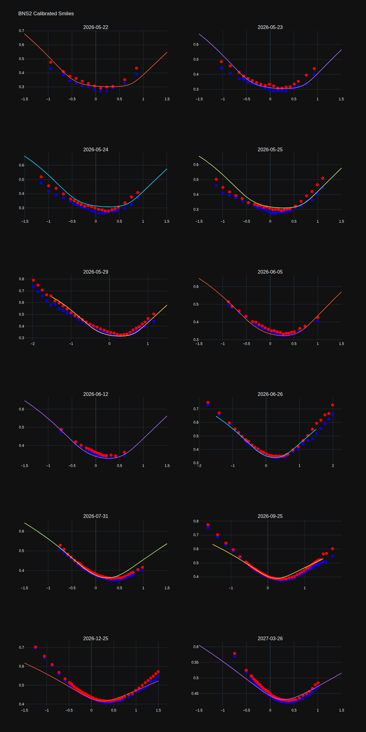
The two-factor variant adds flexibility on the term structure: the fast factor absorbs short-dated skew while the slow factor anchors the long end.
The remaining short-maturity gap is structural in the same way as the single-factor case. BNS2 still injects jumps only through the variance process, so the log-price wings are bounded by the jump sizes scaled by \(|\rho_i|\).
Code
import json

from docs.examples._utils import FIXTURES, assets_path, print_model
from quantflow.options.calibration import BNS2Calibration
from quantflow.options.calibration.base import ResidualKind
from quantflow.options.pricer import OptionPricer, OptionPricingMethod
from quantflow.options.surface import VolSurface, VolSurfaceInputs, surface_from_inputs
from quantflow.sp.bns import BNS, BNS2

# Load a saved volatility surface snapshot and build the surface
with open(FIXTURES / "volsurface_btc.json") as fp:
    surface: VolSurface = surface_from_inputs(VolSurfaceInputs(**json.load(fp)))

surface.bs()
surface.disable_outliers()

# Two-factor BNS: a fast factor for short maturities and a slow one for long.
# Both factors share the same Gamma stationary marginal (vol, decay) following
# the BNS superposition-of-OU construction; only the timescale (kappa) and
# leverage (rho) differ. Opposite-sign leverages lets one factor lift the
# OTM-call wing (rho>0) while the other carries the equity-style downside
# skew (rho<0).
pricer = OptionPricer(
    model=BNS2(
        bns1=BNS.create(vol=0.45, kappa=20.0, decay=10.0, rho=-0.6),
        bns2=BNS.create(vol=0.45, kappa=0.3, decay=10.0, rho=0.3),
        weight=0.5,
    ),
    method=OptionPricingMethod.COS,
)

calibration: BNS2Calibration[BNS2] = BNS2Calibration(
    pricer=pricer,
    vol_surface=surface,
    moneyness_weight=0.3,
    residual_kind=ResidualKind.IV,
)

result = calibration.fit()
print(result.message)
print_model(calibration.model)

fig = calibration.plot_maturities(max_moneyness=1.5, support=101)
fig.update_layout(title="BNS2 Calibrated Smiles")
fig.write_image(assets_path("bns2_calibrated_smile.png"), width=1200)