CIR Process¶

This tutorial shows how to use the CIR (Cox-Ingersoll-Ross) model and validates the analytical marginal PDF against the PDF recovered from the characteristic function.

The model¶

The CIR process is a mean-reverting square-root diffusion with three parameters:

Parameter	Description
`kappa`	Mean-reversion speed
`theta`	Long-run mean
`sigma`	Volatility of volatility
`rate`	Initial value \(x_0\)

from quantflow.sp.cir import CIR

cir = CIR(kappa=2.0, theta=0.5, sigma=0.8, rate=1.0)
print(cir.feller_condition)   # positive: process stays strictly positive
print(cir.is_positive)

The process stays strictly positive when the Feller condition holds:

\[\begin{equation} 2\kappa\theta \geq \sigma^2 \end{equation}\]

Analytical moments¶

The marginal distribution at time \(t\) has closed-form mean and variance, accessible via the marginal:

m = cir.marginal(1.0)
print(m.mean())       # analytical mean
print(m.variance())   # analytical variance

PDF comparison¶

The marginal PDF has two independent routes to the same result:

Analytical: the scaled non-central chi-squared transition density in closed form.
Characteristic function: numerical inversion of \(\Phi = e^{-\phi}\) via pdf_from_characteristic.

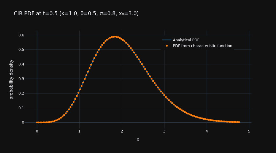
The charts below overlay both for a CIR process with \(\kappa=1\), \(\theta=0.5\), \(\sigma=0.8\), \(x_0=3\), starting well above the long-run mean to make the mean-reversion clearly visible across time horizons.

Short horizon¶

At \(t = 0.5\) the distribution is still centred near the initial value \(x_0\):

Long horizon¶

At \(t = 2.0\) the distribution has mean-reverted toward \(\theta = 0.5\) and the inversion shows visible oscillations:

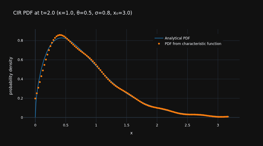
The oscillations are a Gibbs phenomenon. The CIR density has a cusp at the origin: near \(x = 0\) it grows as \(x^{q/2}\) where \(q = 2\kappa\theta/\sigma^2 - 1\). When \(q < 1\) the characteristic function decays algebraically as \(u^{-(1+q/2)}\) rather than exponentially. For these parameters \(q \approx 0.56\), so the integral is still non-negligible when it gets truncated.

At \(t = 0.5\) the mean is nearly three standard deviations from zero, so the cusp is invisible and the inversion is accurate. By \(t = 2\) the process has drifted to within 1.4 standard deviations of the origin and the cusp affects the result.

For CIR with \(q < 1\) the analytical PDF is the right tool. The inversion is confirmed by the characteristic function plot below.

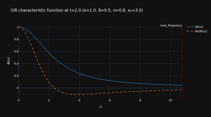
Characteristic function¶

The plot below shows \(|\Phi(u)|\) and \(\text{Re}[\Phi(u)]\) at \(t=2\). The magnitude is still around \(0.05\) at the truncation point, confirming that the integral is cut off before it decays to zero:

Code¶

"""CIR process: compare analytical PDF with PDF from characteristic function."""

import numpy as np
import plotly.graph_objects as go

from docs.examples._utils import assets_path
from quantflow.sp.cir import CIR


def make_figure(cir: CIR, t: float, n: int = 128) -> go.Figure:
    m = cir.marginal(t)
    x = np.linspace(1e-6, m.mean() + 4 * float(m.std()), 300)

    pdf_analytical = cir.analytical_pdf(t, x)
    pdf_cf = m.pdf_from_characteristic(n, simpson_rule=True)

    fig = go.Figure()
    fig.add_trace(
        go.Scatter(
            x=x,
            y=pdf_analytical,
            mode="lines",
            name="Analytical PDF",
            line=dict(color="#1f77b4", width=2),
        )
    )
    fig.add_trace(
        go.Scatter(
            x=pdf_cf.x,
            y=pdf_cf.y,
            mode="markers",
            name="PDF from characteristic function",
            marker=dict(color="#ff7f0e", size=6, symbol="circle"),
        )
    )
    fig.update_layout(
        title=(
            f"CIR PDF at t={t}"
            f" (κ={cir.kappa}, θ={cir.theta}, σ={cir.sigma}, x₀={cir.rate})"
        ),
        xaxis_title="x",
        yaxis_title="probability density",
        legend=dict(x=0.6, y=0.95),
    )
    return fig


def make_cf_figure(cir: CIR, t: float, n: int = 512) -> go.Figure:
    m = cir.marginal(t)
    max_frequency = float(np.asarray(m.frequency_range().ub).flat[0])
    u = np.linspace(0, max_frequency, n)
    cf = cir.characteristic(t, u)

    fig = go.Figure()
    fig.add_trace(
        go.Scatter(
            x=u,
            y=np.abs(cf),
            mode="lines",
            name="|Φ(u)|",
            line=dict(color="#1f77b4", width=2),
        )
    )
    fig.add_trace(
        go.Scatter(
            x=u,
            y=cf.real,
            mode="lines",
            name="Re[Φ(u)]",
            line=dict(color="#ff7f0e", width=2, dash="dash"),
        )
    )
    fig.add_vline(
        x=max_frequency,
        line=dict(color="red", dash="dot", width=1),
        annotation_text="max_frequency",
        annotation_position="top left",
    )
    fig.update_layout(
        title=(
            f"CIR characteristic function at t={t}"
            f" (κ={cir.kappa}, θ={cir.theta}, σ={cir.sigma}, x₀={cir.rate})"
        ),
        xaxis_title="u",
        yaxis_title="Φ(u)",
    )
    return fig


if __name__ == "__main__":
    cir = CIR(kappa=1.0, theta=0.5, sigma=0.8, rate=3.0)

    fig1 = make_figure(cir, t=0.5)
    fig1.write_image(assets_path("cir_pdf_t05.png"), width=900, height=500)

    fig2 = make_figure(cir, t=2.0)
    fig2.write_image(assets_path("cir_pdf_t20.png"), width=900, height=500)

    fig3 = make_cf_figure(cir, t=2.0)
    fig3.write_image(assets_path("cir_cf_t20.png"), width=900, height=500)