SPX Volatility Surface

Build an implied volatility surface for the S&P 500 index from a Yahoo Finance option chain, then calibrate a two-factor BNS model to it.

The Yahoo client fetches the full chain for a ticker. To keep this tutorial offline and reproducible we load a snapshot from a gzipped JSON fixture, but the code is identical to what you would run against the live endpoint.

Loading the chain

Yahoo.loader_from_chain turns the raw chain dictionary into a VolSurfaceLoader. SPX options are non-inverse (quoted in USD) and Yahoo does not provide forwards, so each maturity's forward is recovered from put-call parity inside the loader.

Once the loader has the data, surface() builds the VolSurface, bs() inverts each bid and ask through Black-Scholes, and disable_outliers() drops strikes with unrealistic implied vols.

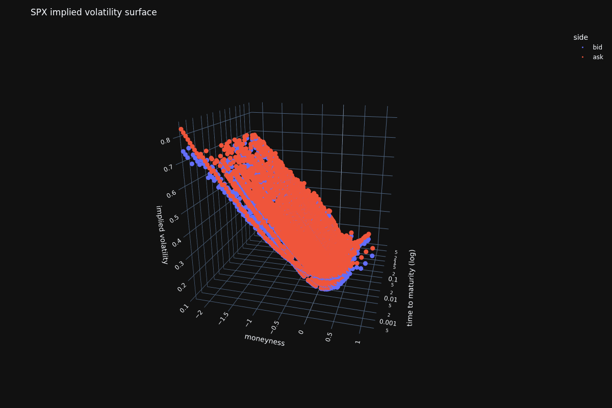
3D surface

plot3d() renders the converged implied vols against moneyness and time to maturity.

BNS2 calibration

A single-factor diffusive Heston struggles on SPX because the short-dated skew is too steep to absorb with a single mean-reversion timescale. BNS2 adds a second Gamma-OU variance factor and injects jumps directly into the variance process, with the leverage parameter mirroring those jumps into the log-price.

BNS2Calibration fits nine parameters with both factors sharing the same Gamma stationary marginal, following the BNS superposition-of-OU construction. See the BNS tutorial for the full parameterisation and the rationale behind tying \((\theta, \beta)\).

The initial parameters seed a fast factor (\(\kappa = 20\)) and a slow factor (\(\kappa = 0.3\)). Both leverages start negative to reflect the persistent equity-style downside skew across the term structure. Residuals are scored in implied-vol space ([ResidualKind.IV][quantflow.options.calibration.base.ResidualKind]) to weight the wings comparably to the ATM region.

Calibrated parameters

xtol termination condition is satisfied.

{
  "bns1": {
    "variance_process": {
      "rate": 0.036657502025866914,
      "kappa": 19.48363847595979,
      "bdlp": {
        "intensity": 0.3725714936418675,
        "jumps": {
          "decay": 10.859007226575585
        }
      }
    },
    "rho": -0.48395745746230767
  },
  "bns2": {
    "variance_process": {
      "rate": 0.036103651402177014,
      "kappa": 0.2794317437198324,
      "bdlp": {
        "intensity": 0.3725714936418675,
        "jumps": {
          "decay": 10.859007226575585
        }
      }
    },
    "rho": -0.2175962129064893
  },
  "weight": 0.5346644440272053
}

The weight collapses almost entirely onto the fast factor, so \(v_0\) for bns1 sits close to the ATM variance read off the 3D surface and bns2 contributes only marginally to the variance level. The slow factor instead carries the stronger negative leverage (\(\rho \approx -0.84\) against the fast factor's \(\rho \approx -0.43\)): its low \(\kappa\) keeps jumps persistent in the log-price, which is what shapes the long-dated downside skew. Both factors share the same BDLP intensity and jump decay by construction.

The remaining short-maturity gap is structural to BNS, as discussed in the BNS tutorial: jumps live in the variance process, so the log-price wings are bounded by the variance jumps scaled by \(|\rho_i|\).

Code

import gzip
import json

from docs.examples._utils import FIXTURES, assets_path, print_model
from quantflow.data.yahoo import Yahoo
from quantflow.options.calibration import BNS2Calibration
from quantflow.options.calibration.base import ResidualKind
from quantflow.options.pricer import OptionPricer, OptionPricingMethod
from quantflow.sp.bns import BNS, BNS2

chain = json.loads(gzip.decompress((FIXTURES / "yahoo_spx.json.gz").read_bytes()))
loader = Yahoo.loader_from_chain(chain, exclude_volume=1)
surface = loader.surface()
surface.bs()
surface.disable_outliers()

fig = surface.plot3d()
fig.update_traces(marker=dict(size=3))
fig.update_layout(
    title="SPX implied volatility surface",
    scene=dict(
        xaxis_title="moneyness",
        yaxis_title="time to maturity (log)",
        zaxis_title="implied volatility",
        yaxis=dict(type="log"),
        camera=dict(eye=dict(x=0.6, y=-2.2, z=0.8)),
    ),
)
fig.write_image(assets_path("spx_vol_surface.png"), width=1200, height=800)

# Calibrate a two-factor BNS model to the SPX surface. A fast factor absorbs
# the steep short-dated equity skew; a slow factor anchors the long end.
pricer = OptionPricer(
    model=BNS2(
        bns1=BNS.create(vol=0.2, kappa=20.0, decay=10.0, rho=-0.6),
        bns2=BNS.create(vol=0.2, kappa=0.3, decay=10.0, rho=-0.3),
        weight=0.5,
    ),
    method=OptionPricingMethod.COS,
)
calibration: BNS2Calibration[BNS2] = BNS2Calibration(
    pricer=pricer,
    vol_surface=surface,
    residual_kind=ResidualKind.IV,
)
result = calibration.fit()
print(result.message)
print_model(calibration.model)

smile = calibration.plot_maturities(max_moneyness=0.5, support=101)
smile.update_layout(title="SPX BNS2 Calibrated Smiles")
smile.write_image(assets_path("spx_vol_surface_bns2.png"), width=1200)