Heston Volatility Model

Calibrating the Heston Model

HestonCalibration fits the five Heston parameters (\(v_0\), \(\theta\), \(\kappa\), \(\sigma\), \(\rho\)) to the implied volatility surface using a two-stage optimisation:

1. L-BFGS-B minimises the scalar cost function (sum of squared weighted price residuals) to reach a good basin of attraction.
2. Trust-region reflective (least_squares with method="trf") refines the solution on the residual vector with tight tolerances and enforces parameter bounds.

Residuals are computed as weight * (model_call_price - mid_call_price) where mid_call_price is the average of the bid and ask call prices.

The weight is \(\min(e^{w \cdot m^2}, w_\text{max})\) controlled by moneyness_weight (the coefficient \(w\)) and max_cost_weight (the cap \(w_\text{max}\)), with \(m = \log(K/F)/\sqrt{T}\) the standardised moneyness. The quadratic exponent matches the gaussian shape of \(1/\nu\) (inverse vega), so a positive moneyness_weight puts wing residuals on the same footing as ATM ones. The cap prevents a single deep-wing option from dominating the loss.

A penalty for violating the Feller condition (\(2\kappa\theta \geq \sigma^2\)) is added during stage 1 to keep the variance process well-behaved.

import json

from docs.examples._utils import FIXTURES, assets_path, print_model
from quantflow.options.calibration import HestonCalibration
from quantflow.options.pricer import OptionPricer, OptionPricingMethod
from quantflow.options.surface import VolSurfaceInputs, surface_from_inputs
from quantflow.sp.heston import Heston

# Load a saved volatility surface snapshot and build the surface
with open(FIXTURES / "volsurface_btc.json") as fp:
    surface = surface_from_inputs(VolSurfaceInputs(**json.load(fp)))

surface.bs()
surface.disable_outliers()

# Create a Heston pricer with initial parameters
pricer = OptionPricer(
    model=Heston.create(vol=0.5, kappa=1, sigma=0.8, rho=0),
    method=OptionPricingMethod.COS,
)

# Set up the calibration, dropping the first (very short) maturity
calibration: HestonCalibration[Heston] = HestonCalibration(
    pricer=pricer,
    vol_surface=surface,
    moneyness_weight=0.3,
)

result = calibration.fit()
print(result.message)
print_model(calibration.model)

# Plot the calibrated smile for all maturities and save as PNG
fig = calibration.plot_maturities(max_moneyness=1.5, support=101)
fig.update_layout(title="Heston Calibrated Smiles")
fig.write_image(assets_path("heston_calibrated_smile.png"), width=1200)

Output

ftol termination condition is satisfied.

{
  "variance_process": {
    "rate": 0.11778702276345798,
    "kappa": 4.13589986171188,
    "sigma": 2.14608395105771,
    "theta": 0.33551094159689643,
    "sample_algo": "implicit"
  },
  "rho": -0.48031281874598625
}

Calibration Options

The moneyness_weight parameter up-weights far-from-the-money options via \(e^{w \cdot m^2}\) where \(m = \log(K/F)/\sqrt{T}\) is the standardised moneyness. The result is capped at max_cost_weight (default 10) so a single deep-wing option cannot dominate the loss.

Plotting the Calibrated Smile

Use plot_maturities() to produce a Plotly figure overlaying market bid/ask implied vols against the model smile for all maturities at once:

fig = calibration.plot_maturities(max_moneyness_ttm=1.5, support=101)
fig.write_image("heston_calibrated_smile.png", width=1200)

The x axis is moneyness.

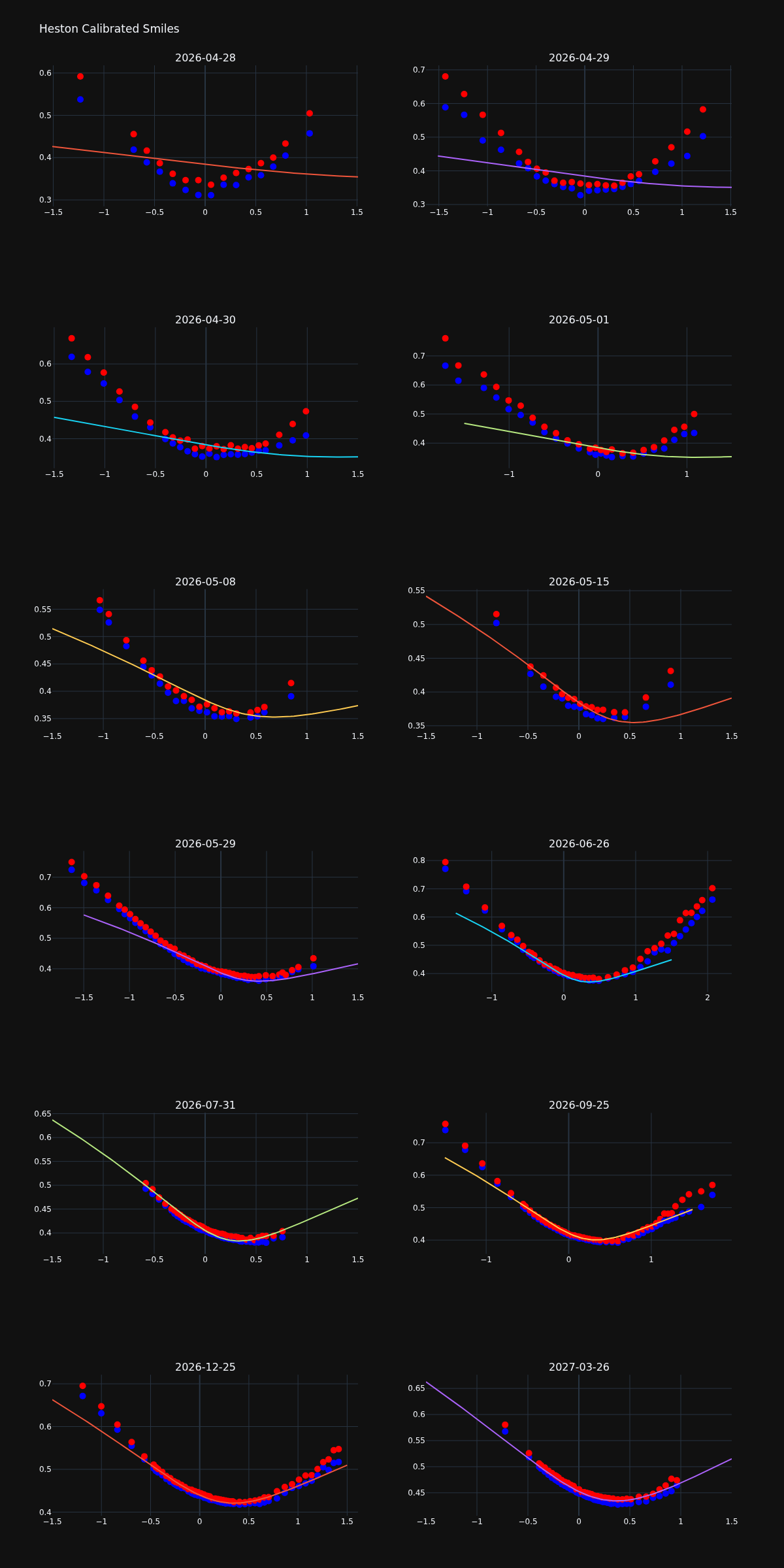
Model Limitations at Short Maturities

Inspecting the calibrated smiles across all maturities reveals a systematic pattern: the Heston model fits long-dated options reasonably well but struggles with short-term maturities, where the market smile is steeper than the model can reproduce.

This is a fundamental structural limitation, not a numerical issue. The Heston model generates an implied volatility smile through two mechanisms: the correlation \(\rho\) between spot and variance (which creates skew) and the volatility-of-variance \(\sigma\) (which inflates the wings). Both effects accumulate diffusively over time. For a maturity \(T\), the smile roughly scales as \(\sigma \sqrt{T}\), so as \(T \to 0\) the distribution collapses toward a Gaussian and the smile flattens.

More precisely, the Heston characteristic function at short maturities satisfies:

\[\begin{equation} \log \phi(u, T) \approx i u \mu T - \tfrac{1}{2} u^2 v_0 T + O(T^2) \end{equation}\]

which is the characteristic function of a Gaussian with variance \(v_0 T\). The higher cumulants that produce skew and excess kurtosis are all \(O(T^2)\) or smaller, so they vanish faster than the Gaussian term as \(T \to 0\).

In practice this means the Heston model essentially reduces to Black-Scholes for near-expiry options. The market, however, exhibits pronounced short-term skew driven by jump risk and the market microstructure of short-dated hedging demand. A diffusion-only model cannot reproduce this behaviour regardless of how its parameters are tuned.

The natural extension is to add a jump component to the dynamics, which contributes a term of order \(O(T)\) to the cumulants and restores the short-term smile. This is the motivation for the Heston jump-diffusion model described in the next section.

Calibrating the Heston Jump-Diffusion Model

HestonJCalibration extends the Heston calibration with a compound Poisson jump component via the HestonJ model. Jumps are drawn from a DoubleExponential distribution, which captures asymmetric jump behaviour common in equity and crypto markets.

import json

from docs.examples._utils import FIXTURES, assets_path, print_model
from quantflow.options.calibration import HestonJCalibration
from quantflow.options.calibration.base import ResidualKind
from quantflow.options.pricer import OptionPricer
from quantflow.options.surface import VolSurface, VolSurfaceInputs, surface_from_inputs
from quantflow.sp.heston import HestonJ
from quantflow.utils.distributions import DoubleExponential
from quantflow.utils.marginal import OptionPricingMethod

# Load a saved volatility surface snapshot and build the surface
with open(FIXTURES / "volsurface_btc.json") as fp:
    surface: VolSurface = surface_from_inputs(VolSurfaceInputs(**json.load(fp)))

surface.bs()
surface.disable_outliers()

# Create a HestonJ pricer with initial parameters
pricer = OptionPricer(
    model=HestonJ.create(
        DoubleExponential,
        vol=0.5,
        kappa=2,
        rho=-0.2,
        sigma=0.8,
        jump_fraction=0.3,
        jump_asymmetry=0.2,
    ),
    method=OptionPricingMethod.COS,
)

# Set up the calibration, dropping the first (very short) maturity
calibration: HestonJCalibration[DoubleExponential] = HestonJCalibration(
    pricer=pricer,
    vol_surface=surface,
    residual_kind=ResidualKind.IV,
)

result = calibration.fit()
print(result.message)
print_model(calibration.model)

# Plot the calibrated smile for all maturities and save as PNG
fig = calibration.plot_maturities(max_moneyness=1.5, support=101)
fig.update_layout(title="HestonJ Calibrated Smiles")
fig.write_image(assets_path("hestonj_calibrated_smile.png"), width=1200)

xtol termination condition is satisfied.

{
  "variance_process": {
    "rate": 0.12916385334299454,
    "kappa": 1.5909761661417188,
    "sigma": 1.082878408144588,
    "theta": 0.1925628047816617,
    "sample_algo": "implicit"
  },
  "rho": -0.2987729884429232,
  "jumps": {
    "intensity": 79.54273026917636,
    "jumps": {
      "decay": 58.835449791869166,
      "loc": 0.007499627395456639,
      "kappa": 1.2119836599641503
    }
  }
}

Plotting the Calibrated Smile

fig = calibration.plot_maturities(max_moneyness_ttm=1.5, support=101)
fig.write_image("hestonj_calibrated_smile.png", width=1200)

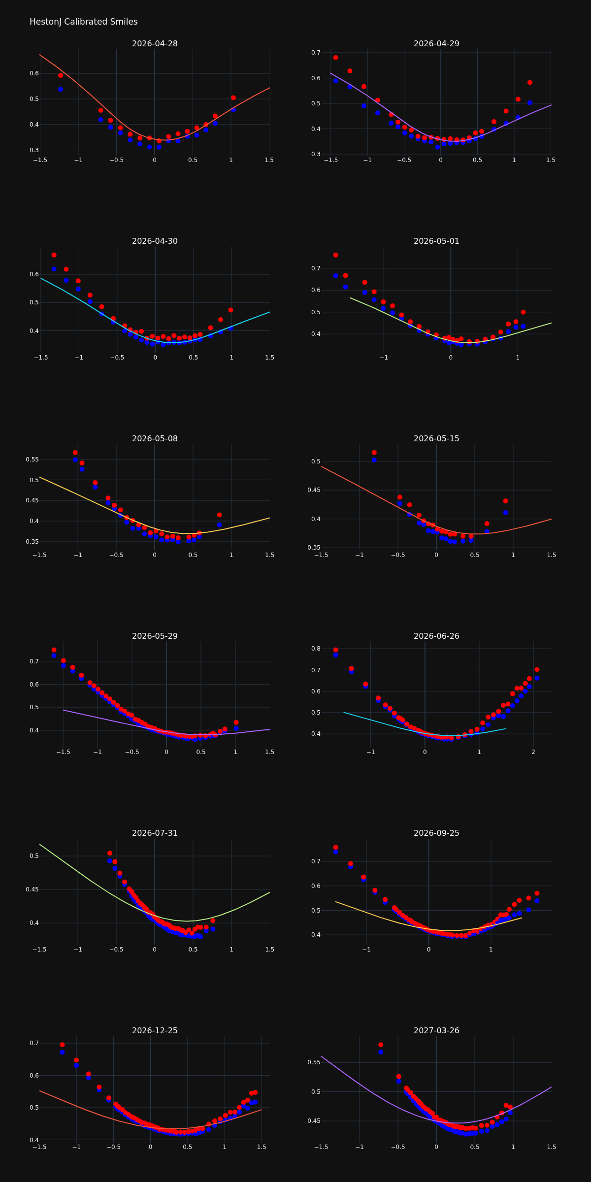
Remaining Limitations at Short Maturities

Adding jumps improves the short-term smile significantly compared to plain Heston, but the fit at the nearest maturities is still imperfect. Several structural reasons combine:

Jump parameters are global. The compound Poisson component has a single intensity \(\lambda\), jump variance, and asymmetry shared across all maturities. Increasing \(\lambda\) to steepen the short-term smile simultaneously distorts the long-term smile, so the optimizer settles on a compromise.

Long maturities dominate the cost function. They have more liquid strikes and therefore more data points. The optimizer minimizes total squared residuals across the whole surface, so short maturities — with fewer strikes — are outvoted and their fit is systematically sacrificed.

The jump distribution is not rich enough. The short-term smile in crypto is driven by large, rare, asymmetric events. A DoubleExponential with fixed parameters cannot simultaneously match the wing curvature at short and long maturities.

The natural next step is a rough volatility model (for example rough Heston with Hurst parameter \(H < \tfrac{1}{2}\)). Because the variance process has long memory and does not behave diffusively at short time scales, rough models produce a steep short-term skew without requiring jumps, and the skew decays as a power law \(T^H\) rather than the \(T^{1/2}\) rate of classical stochastic volatility.

Parameter Reference

The calibrated parameter vector for the jump-diffusion model is:

Parameter	Description
vol	Initial volatility (\(\sqrt{v_0}\))
theta	Long-run volatility (\(\sqrt{\theta}\))
kappa	Mean reversion speed
sigma	Volatility of variance
rho	Spot-variance correlation
jump intensity	Jump arrival rate (jumps per year)
jump variance	Variance of a single jump
jump asymmetry	Asymmetry of the jump distribution (DoubleExponential)