Vasicek Calibration from Rates

This tutorial calibrates the VasicekCurve short-rate model to a panel of historical US Treasury yields by maximum likelihood, using a KalmanFilter to evaluate the likelihood. It shows the full workflow: pulling the data from the Federal Reserve, reshaping it into a uniform panel, fitting the model, and comparing the fitted curve with the observed yields.

For the mechanics of the filter itself, see the Kalman Filter theory page.

The idea

The Vasicek short rate is an Ornstein-Uhlenbeck process. We never observe it directly: what we observe is a cross section of yields at each date. Treating the short rate as a latent state and the yields as noisy linear observations of it turns calibration into a state-space estimation problem.

Over a uniform time step the dynamics reduce to a Gaussian AR(1) and each yield is affine in the short rate. The calibrate_historical_rates method documents these equations. The Kalman filter computes the exact Gaussian log-likelihood of the observed panel, and the calibrator maximises it over \((\kappa, \theta, \sigma, h)\), where \(h\) is the observation noise standard deviation.

Fetching the data

FederalReserve.yield_curves returns the daily Treasury par-yield panel, indexed by date with one column per tenor and rates as decimals. The cached_df helper stores the result as a parquet file so repeated runs do not hit the network.

The calibration assumes a uniform time step, while the raw data is sampled on business days. Resampling to weekly Wednesdays with the average yield over each week gives an evenly spaced panel.

Calibrating

calibrate_historical_rates_dataframe parses the tenor columns into times to maturity, infers the time step from the index, converts the par yields to continuously compounded rates (here frequency=2 for semiannual compounding), and runs the maximum-likelihood fit. One full Kalman pass over the panel is performed per optimiser iteration.

The fitted parameters and the final filtered short rate are returned on the calibrated curve:

{
  "curve_type": "vasicek_curve",
  "rate": "0.0401793039",
  "kappa": "0.2636482462",
  "theta": "0.0718445057",
  "sigma": "0.0613955961"
}

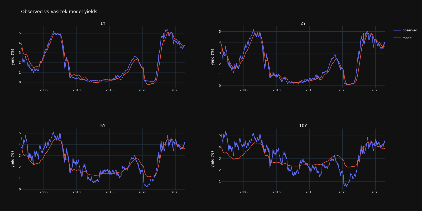
Model versus observed through time

The fit is a time-series fit, so the right check is whether the model tracks the history of each tenor. The calibrator exposes the filtered_short_rate path, from which each tenor's model-implied yield is reconstructed through the affine yield relation and plotted against its observed history.

The single factor tracks the short and intermediate tenors (1Y, 2Y) closely, but the model yields are smoother than the data at the long end (5Y, 10Y): one mean-reverting factor cannot capture the independent variation of the long end, the expected limitation of the one-factor Vasicek model.

Code

import asyncio
from datetime import timedelta

import numpy as np
import pandas as pd
import plotly.graph_objects as go
from plotly.subplots import make_subplots

from docs.examples._utils import assets_path, cached_df
from quantflow.data.fed import FederalReserve
from quantflow.rates.calibration import tenor_to_years
from quantflow.rates.vasicek import VasicekCurve


@cached_df(ttl=timedelta(days=1))
def fed_yield_curves() -> pd.DataFrame:
    async def fetch() -> pd.DataFrame:
        async with FederalReserve() as fed:
            return await fed.yield_curves()

    return asyncio.run(fetch())


# daily par-yield panel from the Federal Reserve (cached for a day)
df = fed_yield_curves()
# weekly panel (uniform 7-day step) using the average yield over each week
weekly = df.resample("W-WED").mean().dropna()

# calibrate the Vasicek short-rate model to the panel by Kalman-filter MLE
calibrator = VasicekCurve().calibrator()
curve = calibrator.calibrate_historical_rates_dataframe(weekly, frequency=2)
print(curve.model_dump_json(indent=2, exclude={"ref_date"}))

# rebuild model-implied yields from the filtered short rate path: y = (B r - A) / tau
ttm = np.array([tenor_to_years(c) for c in weekly.columns])
a, b = curve.affine_coefficients(ttm)
A, B = np.asarray(a, dtype=float), np.asarray(b, dtype=float)
short_rate = calibrator.filtered_short_rate  # one value per observation date

# observed (par -> continuous) and model yields per tenor, over time
tenors = ["1Y", "2Y", "5Y", "10Y"]
fig = make_subplots(rows=2, cols=2, subplot_titles=tenors)
for k, tenor in enumerate(tenors):
    i = weekly.columns.get_loc(tenor)
    observed = 2.0 * np.log1p(weekly[tenor].to_numpy() / 2.0) * 100
    model = (B[i] * short_rate - A[i]) / ttm[i] * 100
    row, col = k // 2 + 1, k % 2 + 1
    fig.add_trace(
        go.Scatter(
            x=weekly.index,
            y=observed,
            name="observed",
            legendgroup="observed",
            showlegend=k == 0,
            line=dict(color="#636efa"),
        ),
        row=row,
        col=col,
    )
    fig.add_trace(
        go.Scatter(
            x=weekly.index,
            y=model,
            name="model",
            legendgroup="model",
            showlegend=k == 0,
            line=dict(color="#ef553b"),
        ),
        row=row,
        col=col,
    )
fig.update_layout(title="Observed vs Vasicek model yields")
fig.update_yaxes(title_text="yield (%)")
fig.write_image(assets_path("rates_kalman.png"), width=1600, height=800)