Discount Curves from Option Prices

Every implied volatility on a surface is inverted against a forward price. The forward at each maturity is determined by the option market itself, and getting it wrong corrupts every single volatility on the surface.

The central principle of this tutorial is simple: for a smooth implied volatility surface, the forwards must be calculated from put-call parity. The sections below show what goes wrong with any other forward, how parity identifies the right one, and how the quantflow calibration implements the principle: calibrate_forwards estimates the forwards first, and calibrate_curves derives the discount curves from them. Everything is demonstrated on a recorded snapshot of the BTC option book from Deribit. It is the reference for the calibration design going forward. See Forwards and Discount Factors for the underlying theory.

The data

The snapshot was recorded on 1 August 2026 and is rebuilt offline with loader_from_book. The exact reference time appears in the chart titles. It contains 13 maturities, a listed future at every maturity, and the perpetual as spot. Several hundred option quotes carry both the call and the put side, so put-call parity can be observed directly.

The problem: a wrong forward

Implied volatilities are inverted from out of the money quotes: puts below the forward, calls above.

An option price is the sum of intrinsic value and time value. Only the time value carries volatility information. An out of the money option has no intrinsic value, so its whole price is time value.

An in the money option still has meaningful time value near the money. But the deeper it moves in the money, the more intrinsic value dominates its price. The inversion then extracts a small time value from a large price, and quote noise swings the implied volatility. By put-call parity the out of the money option at the same strike carries the same information, with far better conditioning. Market liquidity concentrates out of the money for the same reason.

The forward therefore matters twice. It enters the Black formula, and before that it decides which side of each strike is out of the money. The two sides meet at the forward. If the inversion uses a forward that disagrees with the option market, they disagree exactly there: with a forward that is too low, the calls come out too high and the puts too low.

The chart below inverts the same mid quotes twice. The left panel uses the spot price as forward and the smile breaks at the switch. The right panel uses the listed future and the smile is continuous.

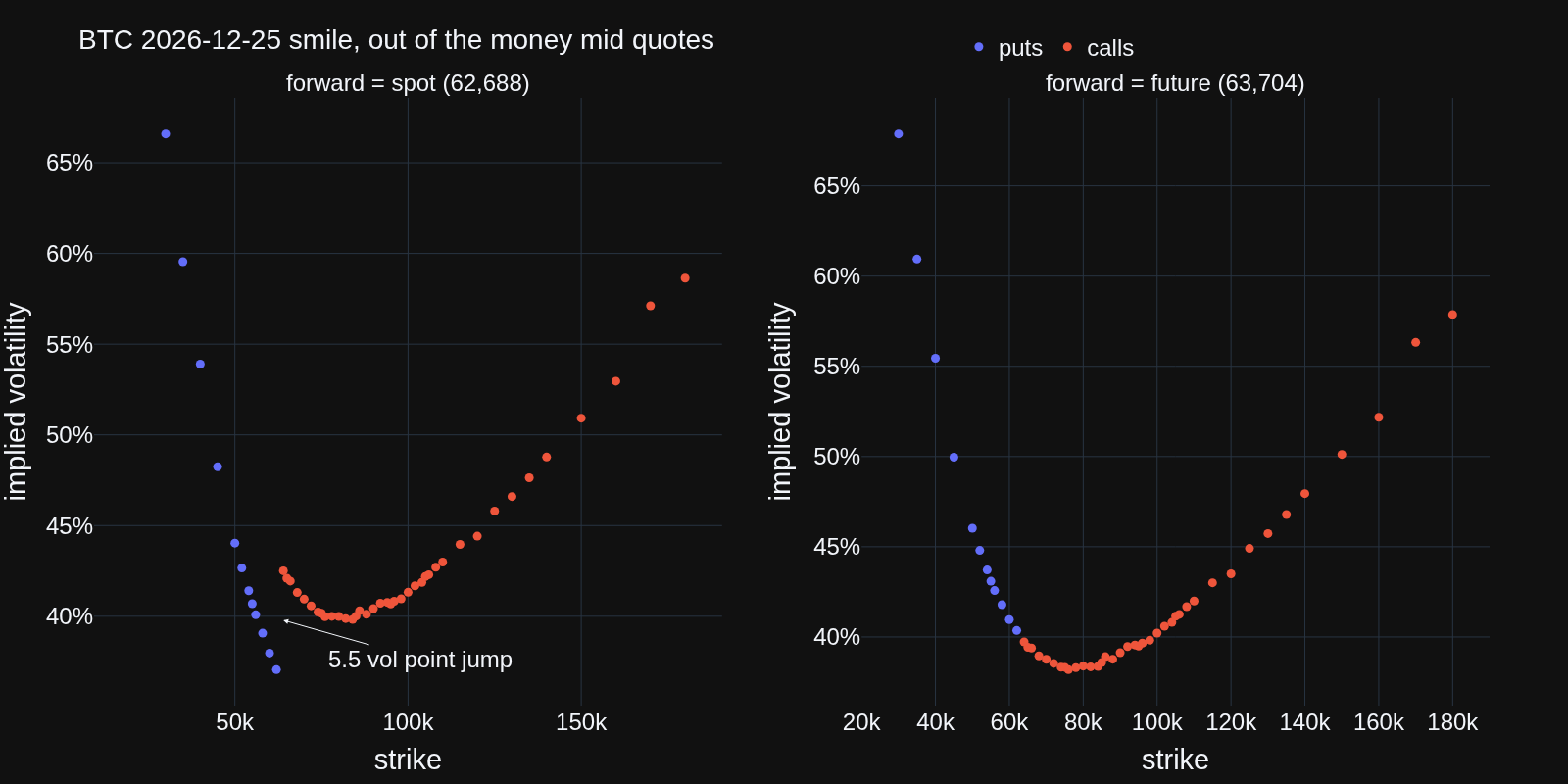
The jump is the forward error expressed in volatility units, so it grows with the time to maturity. The spot is an extreme case, but the mechanism is general. Any forward that deviates from the one embedded in the option quotes leaves a jump at the switch, in proportion to the deviation. The question is therefore how to find the forward the option market itself is using. That is the fix section below.

What the library does. calibrate_forwards estimates the parity forward of every maturity and stores it on the cross section. The surface then prices each cross section off its pricing_forward: the parity forward when calibrated, the market forward of the cross section otherwise. Discount curves are never used to derive pricing forwards.

The check to remember. A jump in the smile where puts switch to calls is always the signature of a wrong forward. A correct calibration makes the two sides meet, whatever curve model is used.

Quote selection

The choice of which side to invert at each strike is controlled by OptionSelection.

OTM selects the out of the money side, with the switch at the forward. CALL, PUT and ALL select fixed sides and are mostly diagnostic tools. Comparing the CALL and PUT smiles at the same strikes is another way to detect a wrong forward.

BEST currently selects the out of the money side and blends the call and put implied volatilities near the money. The blending smooths a small residual basis, but it cannot repair a wrong forward.

This tutorial assumes plain out of the money selection throughout.

What remains open. Placing the switch at the raw forward is itself a simplification. The natural coordinate for the boundary is the vol adjusted moneyness, or its convexity adjusted variant. Both measure the distance from the money in units of standard deviation. They require the implied volatility, which is not known before the first inversion. A solid BEST strategy therefore needs two passes: invert with the plain out of the money selection first, then re-select the quotes using the fitted volatilities and invert again. This strategy still needs to be devised, implemented, and documented here.

The fix: forwards from parity

The forward the option market is using is written in the option quotes themselves. For every strike \(K\) quoted on both sides, put-call parity links the mid prices to the two discount factors:

\[\begin{equation} C - P = D_a S - D_q K \end{equation}\]

Within one maturity this is a straight line in the strike. The chart below shows the regression at two maturities of the snapshot: the front maturity on the left and a long maturity on the right, each titled with its date and time to maturity. The dashed vertical lines mark where each regression line crosses zero, which is the parity implied forward.

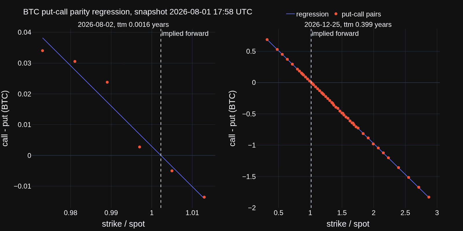
The long maturity is textbook: dozens of pairs, a strike range spanning three times the spot, and quotes that sit exactly on the line. The front maturity is a preview of the problems ahead: a handful of pairs, a strike range of a few percent, and visible scatter around the line.

The zero crossing is the strike at which the parity line crosses zero, visible in the chart above where the regression line meets the horizontal axis. At that strike the call and the put have the same price. Setting \(C - P = 0\) in the equation above gives \(K = S D_a / D_q\), which is the forward \(F\).

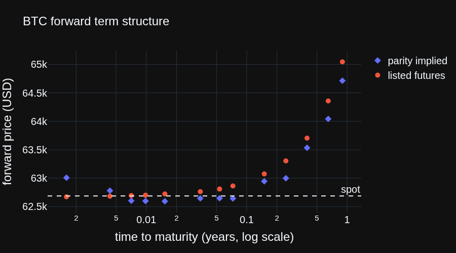
This strike sits inside the quoted range, so it is found by interpolating between quotes, never by extrapolating. The parity implied forward is therefore extremely well identified. And it does not have to agree with the listed future.

The term structure below compares the two, with the time to maturity on a log scale to spread out the front.

Not all parity pairs deserve the same trust. The same regressions are shown below in moneyness terms, computed against the spot since the forward is not known yet. Moneyness measures the distance from the money in square root of time units, so the two maturities become comparable on this axis.

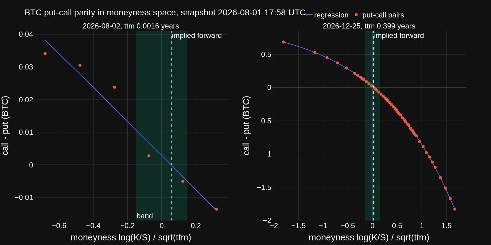
A pair far from the money contains one option that is deep in the money. Its quote is dominated by intrinsic value, tick rounding and bid ask spread, for the same reasons discussed for the smile inversion. Those pairs drag the regression away from the money, which is exactly where the zero crossing lives. The shaded band keeps only pairs near the money.

What the library does. calibrate_forward implements this as an iterative weighted regression. Each pair is weighted by the inverse of its parity bid ask spread, so noisy pairs count less: this is the data driven core of the estimator. On top of the weights, pairs are selected inside a band of convexity adjusted moneyness, one standard deviation by default, widened automatically when too few pairs survive. The band coordinates require the forward and the volatility, so the algorithm iterates: fit the crossing, estimate the at the money volatility from the nearest straddle, re-select, refit. Two or three iterations suffice.

calibrate_forwards runs the estimator at every maturity and stores the forwards on the cross sections, where the surface picks them up for pricing.

The chart below shows the result: a naive regression over all pairs drifts from the listed futures by up to half a percent, while the calibrated forwards agree with them within a few basis points at every maturity, including the noisy front.

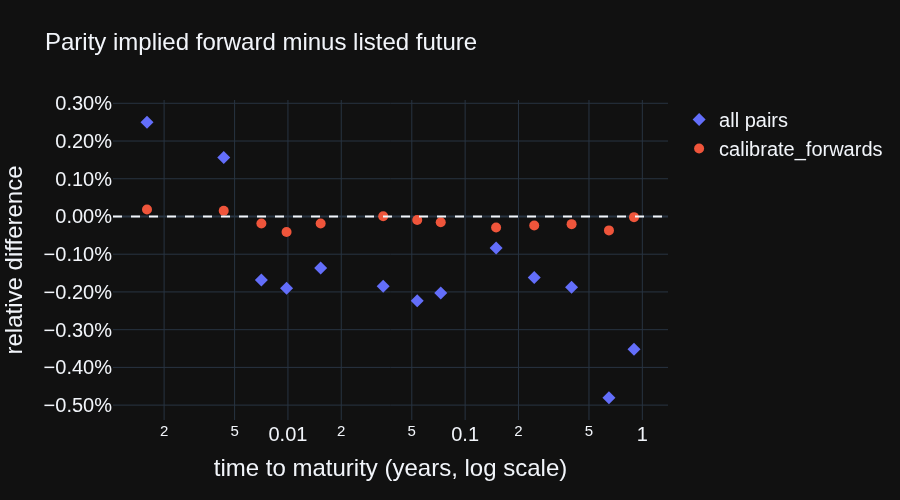
The choice of the band width is not critical, which is the point of the weighted design. On this snapshot the maximum error against the listed futures moves only between 4 and 8 basis points as the band varies from half to three standard deviations, against 48 basis points for the unweighted all pairs regression.

The discount factor split

The parity line pins down the forward with high precision. The split of the line into \(D_a\) and \(D_q\) is a different story. It requires the intercept \(D_a S\), which lives at \(K = 0\), far outside any quoted strike. Extrapolating there is ill-conditioned. Small quote noise moves both discount factors a lot, in opposite directions.

What the library does. calibrate_curves never fits the two discount factors freely. It calibrates the forwards first, then estimates a single parameter per maturity, the quote discount factor, with the forward held fixed (quote_discount). The asset discount factor follows from the forward formula:

\[\begin{equation} D_a = D_q \frac{F}{S} \end{equation}\]

The selected curve models are then fitted to those discount factors: a parametric model pools all maturities while an interpolated curve passes through them. This guarantees that the curves are consistent with the parity forwards, and since the surface prices off the parity forwards directly, the smile cannot break whatever curve model is selected.

Short maturities

The forward of a short maturity is well identified: the crossing is an interpolation and the front forwards above agree with the futures within basis points. The discounting of a short maturity is not. The quote discount factor is the slope of the parity line, and a chain that expires in hours quotes strikes only a few percent apart, so the slope estimate carries an error of percents. In rate units the damage is then amplified:

\[\begin{equation} r(\tau) = -\frac{\ln D(\tau)}{\tau} \end{equation}\]

A two percent discount factor error at three weeks is already a forty percent zero rate error. This is not an estimation problem to fix: a chain of short dated options simply contains no information about discounting.

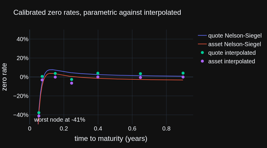
What the library does. calibrate_curves excludes maturities below min_ttm (two weeks by default) from the curve fitting. Their forwards are still calibrated and used for pricing; their discounting extrapolates from the first calibrated node, which is essentially exact since the discount factor of a few days is one within basis points.

The chart below shows the calibrated zero rates. The interpolated nodes scatter at the short end even after the exclusion, while the parametric curves pool the maturities. Rates implied from options become meaningful roughly beyond a month.

Summary

Problem	Effect	Solution
Wrong forward	Smile jumps at the put to call switch	Forwards calibrated from parity, used directly for pricing
Parity pairs far from the money	Deep in the money leg drags the implied forward	Inverse spread weights and an adaptive moneyness band
Weak identification of the split	Freely fitted curves absorb quote noise	One parameter per maturity with the forward held fixed
Short maturity discounting	Front zero rates unidentifiable	Maturities below min_ttm excluded from curve fitting
Switch at the raw forward	Selection ignores the volatility scale	Open: two pass selection in vol adjusted moneyness

The only open item is the two pass BEST selection of the quote selection section. Everything else in this table is implemented by calibrate_forwards and calibrate_curves.

Code

from typing import cast

import numpy as np
import pandas as pd
import plotly.graph_objects as go
from plotly.subplots import make_subplots

from docs.examples._utils import assets_path, btc_surface_loader
from quantflow.options.bs import implied_black_volatility
from quantflow.options.surface import VolCrossSection
from quantflow.rates import InterpolatedMonotonicCubicCurve, NelsonSiegelCurve

MATURITY = "2026-12-25"


def style(fig: go.Figure, font_size: int = 20) -> go.Figure:
    """Apply a readable font scale to a figure"""
    fig.update_layout(font_size=font_size, title_font_size=font_size + 4)
    fig.update_annotations(font_size=font_size)
    return fig


def smile(cross: VolCrossSection, forward: float, ttm: float) -> pd.DataFrame:
    """Invert out of the money mid quotes with the given forward price"""
    strikes, ks, prices, cps = [], [], [], []
    for sk in cross.strikes:
        strike = float(sk.strike)
        option = sk.put if strike <= forward else sk.call
        if option is None:
            continue
        strikes.append(strike)
        ks.append(np.log(strike / forward))
        # inverse options are quoted in BTC, already in forward space
        prices.append(float(option.bid.price + option.ask.price) / 2)
        cps.append(-1.0 if strike <= forward else 1.0)
    result = implied_black_volatility(
        k=np.array(ks),
        price=np.array(prices),
        ttm=np.full(len(ks), ttm),
        initial_sigma=np.full(len(ks), 0.5),
        call_put=np.array(cps),
    )
    frame = pd.DataFrame(
        dict(
            strike=strikes,
            iv=np.asarray(result.values).ravel(),
            side=["put" if cp < 0 else "call" for cp in cps],
        )
    )
    return frame[np.asarray(result.converged).ravel()]


def smile_panel(fig: go.Figure, frame: pd.DataFrame, col: int) -> None:
    for side, color in (("put", "#636efa"), ("call", "#ef553b")):
        data = frame[frame.side == side]
        fig.add_trace(
            go.Scatter(
                x=data.strike,
                y=data.iv,
                mode="markers",
                marker=dict(symbol="circle", color=color, size=9),
                name=f"{side}s",
                showlegend=col == 1,
            ),
            row=1,
            col=col,
        )


loader = btc_surface_loader()
surface = loader.surface()
ref_date = surface.ref_date
spot = float(surface.spot_price())

cross = next(c for c in surface.maturities if str(c.maturity.date()) == MATURITY)
ttm = cross.ttm(ref_date)
future = float(cross.forward.mid)

# figure 1: the same quotes inverted with the spot and with the market future
fig = make_subplots(
    rows=1,
    cols=2,
    subplot_titles=(
        f"forward = spot ({spot:,.0f})",
        f"forward = future ({future:,.0f})",
    ),
)
bad = smile(cross, spot, ttm)
smile_panel(fig, bad, 1)
smile_panel(fig, smile(cross, future, ttm), 2)
last_put = bad[bad.side == "put"].iloc[-1]
first_call = bad[bad.side == "call"].iloc[0]
jump = first_call.iv - last_put.iv
fig.add_annotation(
    x=first_call.strike,
    y=(first_call.iv + last_put.iv) / 2,
    xref="x1",
    yref="y1",
    text=f"{100 * jump:.1f} vol point jump",
    showarrow=True,
    arrowhead=2,
    ax=140,
    ay=40,
)
fig.update_layout(
    title=f"BTC {MATURITY} smile, out of the money mid quotes",
    legend=dict(x=0.62, y=1.12, orientation="h"),
)
fig.update_xaxes(title_text="strike")
fig.update_yaxes(title_text="implied volatility", tickformat=".0%")
style(fig, font_size=24)
fig.write_image(assets_path("curve_calibration_smile.png"), width=1600, height=800)


# figure 2: put-call parity regression at the front and at a long maturity
def parity_panel(fig: go.Figure, cross: VolCrossSection, col: int) -> None:
    """Add the parity regression of one maturity to a subplot column"""
    section = loader.maturities[cross.maturity]
    parities = section.put_call_parities(
        surface.spot_price(), ref_date=ref_date, max_pairs=100
    )
    cp = parities.regressand()
    k = parities.regressor()
    slope, intercept = np.polyfit(k, cp, 1)
    # the forward is the strike where the regression line crosses zero
    zero_crossing = -intercept / slope
    k_line = np.linspace(k.min(), k.max(), 50)
    fig.add_trace(
        go.Scatter(
            x=k_line,
            y=intercept + slope * k_line,
            mode="lines",
            line=dict(color="#636efa"),
            name="regression",
            showlegend=col == 1,
        ),
        row=1,
        col=col,
    )
    fig.add_trace(
        go.Scatter(
            x=k,
            y=cp,
            mode="markers",
            marker=dict(symbol="circle", size=10, color="#ef553b"),
            name="put-call pairs",
            showlegend=col == 1,
        ),
        row=1,
        col=col,
    )
    fig.add_vline(
        x=zero_crossing,
        line_dash="dash",
        annotation_text="implied forward",
        row=1,
        col=col,
    )


front = surface.maturities[0]
front_ttm = front.ttm(ref_date)
fig = make_subplots(
    rows=1,
    cols=2,
    subplot_titles=(
        f"{front.maturity.date()}, ttm {front_ttm:.4f} years",
        f"{cross.maturity.date()}, ttm {ttm:.3f} years",
    ),
)
parity_panel(fig, front, 1)
parity_panel(fig, cross, 2)
fig.update_layout(
    title=f"BTC put-call parity regression, snapshot {ref_date:%Y-%m-%d %H:%M} UTC",
    legend=dict(x=0.62, y=1.12, orientation="h"),
)
fig.update_xaxes(title_text="strike / spot")
fig.update_yaxes(title_text="call - put (BTC)")
style(fig, font_size=24)
fig.write_image(assets_path("curve_calibration_parity.png"), width=1600, height=800)

# figure 3: the same parity regressions in moneyness space
BAND = 0.15


def parity_moneyness_panel(fig: go.Figure, cross: VolCrossSection, col: int) -> None:
    """Add the parity regression of one maturity in moneyness space"""
    section = loader.maturities[cross.maturity]
    parities = section.put_call_parities(
        surface.spot_price(), ref_date=ref_date, max_pairs=100
    )
    cp = parities.regressand()
    k = parities.regressor()
    ttm_cross = cross.ttm(ref_date)
    m = np.log(k) / np.sqrt(ttm_cross)
    slope, intercept = np.polyfit(k, cp, 1)
    zero_crossing = -intercept / slope
    m_line = np.linspace(m.min(), m.max(), 100)
    fig.add_trace(
        go.Scatter(
            x=m_line,
            y=intercept + slope * np.exp(m_line * np.sqrt(ttm_cross)),
            mode="lines",
            line=dict(color="#636efa"),
            name="regression",
            showlegend=col == 1,
        ),
        row=1,
        col=col,
    )
    fig.add_trace(
        go.Scatter(
            x=m,
            y=cp,
            mode="markers",
            marker=dict(symbol="circle", size=10, color="#ef553b"),
            name="put-call pairs",
            showlegend=col == 1,
        ),
        row=1,
        col=col,
    )
    fig.add_vline(
        x=float(np.log(zero_crossing) / np.sqrt(ttm_cross)),
        line_dash="dash",
        annotation_text="implied forward",
        row=1,
        col=col,
    )
    annotation = (
        dict(annotation_text="band", annotation_position="bottom left")
        if col == 1
        else {}
    )
    fig.add_vrect(
        x0=-BAND,
        x1=BAND,
        fillcolor="#00cc96",
        opacity=0.15,
        line_width=0,
        row=1,
        col=col,
        **annotation,
    )


fig = make_subplots(
    rows=1,
    cols=2,
    subplot_titles=(
        f"{front.maturity.date()}, ttm {front_ttm:.4f} years",
        f"{cross.maturity.date()}, ttm {ttm:.3f} years",
    ),
)
parity_moneyness_panel(fig, front, 1)
parity_moneyness_panel(fig, cross, 2)
fig.update_layout(
    title=(
        f"BTC put-call parity in moneyness space, "
        f"snapshot {ref_date:%Y-%m-%d %H:%M} UTC"
    ),
    legend=dict(x=0.62, y=1.12, orientation="h"),
)
fig.update_xaxes(title_text="moneyness log(K/S) / sqrt(ttm)")
fig.update_yaxes(title_text="call - put (BTC)")
style(fig, font_size=24)
fig.write_image(
    assets_path("curve_calibration_parity_moneyness.png"), width=1600, height=800
)

# figure 4: forward term structure, market futures against parity implied forwards
term = loader.implied_forward_term_structure(max_pairs=100)
implied = pd.DataFrame(term, columns=["maturity", "ttm", "forward"])
futures = pd.DataFrame(
    dict(
        ttm=[c.ttm(ref_date) for c in surface.maturities],
        forward=[float(c.forward.mid) for c in surface.maturities],
    )
)
fig = go.Figure()
fig.add_trace(
    go.Scatter(
        x=implied.ttm,
        y=implied.forward,
        mode="markers",
        marker=dict(symbol="diamond", size=10),
        name="parity implied",
    )
)
fig.add_trace(
    go.Scatter(
        x=futures.ttm,
        y=futures.forward,
        mode="markers",
        marker=dict(symbol="circle", size=10),
        name="listed futures",
    )
)
fig.add_hline(y=spot, line_dash="dash", annotation_text="spot")
fig.update_layout(
    title="BTC forward term structure",
    xaxis_title="time to maturity (years, log scale)",
    xaxis_type="log",
    yaxis_title="forward price (USD)",
)
style(fig)
fig.write_image(assets_path("curve_calibration_forwards.png"), width=900, height=500)

# figure 5: the parity forward error against the listed future, with a naive
# all pairs regression and with the calibrate_forwards algorithm
rows = []
for c in surface.maturities:
    section = loader.maturities[c.maturity]
    parities = section.put_call_parities(
        surface.spot_price(), ref_date=ref_date, max_pairs=100
    )
    cp_pairs = parities.regressand()
    k_pairs = parities.regressor()
    slope, intercept = np.polyfit(k_pairs, cp_pairs, 1)
    rows.append(dict(ttm=c.ttm(ref_date), forward=-intercept / slope * spot))
naive = pd.DataFrame(rows)
parity_forwards = loader.calibrate_forwards()
calibrated = pd.DataFrame(
    dict(
        ttm=[entry[1] for entry in parity_forwards],
        forward=[float(entry[2]) for entry in parity_forwards],
    )
)
fig = go.Figure()
for name, symbol, frame in (
    ("all pairs", "diamond", naive),
    ("calibrate_forwards", "circle", calibrated),
):
    merged = frame.merge(futures, on="ttm", suffixes=("", "_future"))
    fig.add_trace(
        go.Scatter(
            x=merged.ttm,
            y=(merged.forward - merged.forward_future) / merged.forward_future,
            mode="markers",
            marker=dict(symbol=symbol, size=10),
            name=name,
        )
    )
fig.add_hline(y=0, line_dash="dash")
fig.update_layout(
    title="Parity implied forward minus listed future",
    xaxis_title="time to maturity (years, log scale)",
    xaxis_type="log",
    yaxis_title="relative difference",
    yaxis_tickformat=".2%",
)
style(fig)
fig.write_image(
    assets_path("curve_calibration_forward_basis.png"), width=900, height=500
)

# figure 6: parametric curves pool information across maturities, interpolated
# curves fit one node per maturity and amplify the noise at the front
loader_ns = btc_surface_loader()
loader_ns.calibrate_curves(quote_curve=NelsonSiegelCurve, asset_curve=NelsonSiegelCurve)
loader_in = btc_surface_loader()
loader_in.calibrate_curves(
    quote_curve=InterpolatedMonotonicCubicCurve,
    asset_curve=InterpolatedMonotonicCubicCurve,
)
quote_in = cast(InterpolatedMonotonicCubicCurve, loader_in.quote_curve)
asset_in = cast(InterpolatedMonotonicCubicCurve, loader_in.asset_curve)
max_ttm = max(float(c.ttm(ref_date)) for c in surface.maturities)
ttm_grid = np.linspace(1 / 52, max_ttm, 100)
node_ttm = np.array(
    [
        (date - ref_date).total_seconds() / (365 * 86400)
        for date in quote_in.anchor_dates
    ]
)
fig = go.Figure()
for name, curve in (("quote", loader_ns.quote_curve), ("asset", loader_ns.asset_curve)):
    fig.add_trace(
        go.Scatter(
            x=ttm_grid,
            y=np.atleast_1d(curve.continuously_compounded_rate(ttm_grid)),
            mode="lines",
            name=f"{name} Nelson-Siegel",
        )
    )
for name, curve in (("quote", quote_in), ("asset", asset_in)):
    fig.add_trace(
        go.Scatter(
            x=node_ttm,
            y=[float(r) for r in curve.anchor_rates],
            mode="markers",
            marker=dict(symbol="circle", size=10),
            name=f"{name} interpolated",
        )
    )
node_rates = [float(r) for curve in (quote_in, asset_in) for r in curve.anchor_rates]
worst = min(node_rates, key=lambda r: -abs(r))
off_scale = sum(1 for r in node_rates if abs(r) > 0.5)
fig.update_layout(
    title="Calibrated zero rates, parametric against interpolated",
    xaxis_title="time to maturity (years)",
    yaxis_title="zero rate",
    yaxis_tickformat=".0%",
    yaxis_range=[-0.5, 0.5],
)
note = (
    f"{off_scale} front nodes off scale, worst at {worst:.0%}"
    if off_scale
    else f"worst node at {worst:.0%}"
)
fig.add_annotation(x=0.02, y=-0.45, text=note, showarrow=False, xanchor="left")
style(fig)
fig.write_image(assets_path("curve_calibration_rates.png"), width=900, height=500)

# structured output: calibrated parity forwards against market futures
table = calibrated.merge(futures, on="ttm", suffixes=("_parity", "_future"))
table.insert(0, "maturity", [str(entry[0].date()) for entry in parity_forwards])
table["basis"] = table.forward_parity - table.forward_future
table = table.round(dict(ttm=3, forward_parity=1, forward_future=1, basis=1))
print(table.to_string(index=False))

  maturity   ttm  forward_parity  forward_future  basis
2026-08-02 0.002         62684.2         62672.5   11.7
2026-08-03 0.004         62692.0         62682.5    9.5
2026-08-04 0.007         62683.4         62695.0  -11.6
2026-08-05 0.010         62674.1         62700.0  -25.9
2026-08-07 0.015         62712.1         62723.8  -11.6
2026-08-14 0.034         62764.1         62763.8    0.4
2026-08-21 0.054         62802.8         62808.8   -5.9
2026-08-28 0.073         62854.0         62863.8   -9.7
2026-09-25 0.150         63056.5         63075.0  -18.5
2026-10-30 0.245         63288.5         63303.8  -15.2
2026-12-25 0.399         63690.8         63703.8  -13.0
2027-03-26 0.648         64333.8         64357.5  -23.7
2027-06-25 0.897         65043.9         65045.0   -1.1